The data.table R package

For most cases, the most proper data wrangling tool in R is the dplyr package. Nonetheless, when dealing with large amounts of data, the data.table package is the fastest alternative available for doing data processing within R (see the benchmarks).

Reading and Writing Data

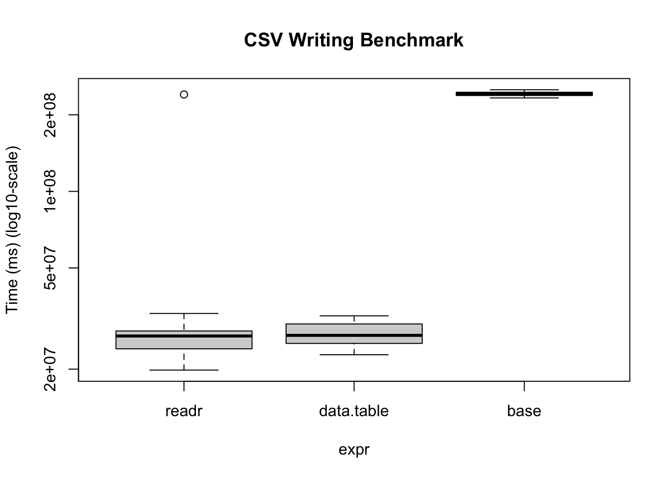
Reading and writing operations with data.table’s fread and fwrite are highly optimized. Here is a benchmark we can do on our own:

library(readr) # tidyverse's
library(data.table)
library(microbenchmark)

# Generating a large dataset of random numbers
set.seed(1231)
x <- runif(5e4 * 10) |> matrix(ncol = 10) |> data.frame()

# Creating tempfiles
temp_dt <- tempfile(fileext = ".csv")
temp_tv <- tempfile(fileext = ".csv")
temp_r  <- tempfile(fileext = ".csv")

bm <- microbenchmark(
  readr      = write_csv(x, temp_tv, num_threads = 1L, progress = FALSE),
  data.table = fwrite(
    x, temp_dt, verbose = FALSE, nThread = 1L,
    showProgress = FALSE),
  base       = write.csv(x, temp_r),
  times = 20
)

Warning in microbenchmark(readr = write_csv(x, temp_tv, num_threads = 1L, :
less accurate nanosecond times to avoid potential integer overflows

bm

Unit: milliseconds
       expr       min        lq      mean    median        uq       max neval
      readr  19.83141  24.03928  36.83226  26.99321  28.25456 240.43183    20
 data.table  22.78067  25.24101  27.63036  27.15459  30.10759  32.39791    20
       base 233.02502 238.19760 241.98725 242.07634 245.42001 250.93275    20

# We can also visualize it
bm |>
  plot(
    log = "y",
    ylab = "Time (ms) (log10-scale)",
    main = "CSV Writing Benchmark"
  )

The same thing applies when reading data

# Writing the data
fwrite(x, temp_r, verbose = FALSE, nThread = 1L, showProgress = FALSE)

# Benchmarking
bm <- microbenchmark(
  readr      = read_csv(
    temp_r, progress = FALSE, num_threads = 1L,
    show_col_types = FALSE
    ),
  data.table = fread(
    temp_r, verbose = FALSE, nThread = 1L,
    showProgress = FALSE
    ),
  base       = read.csv(temp_r),
  times = 10
)

bm

Unit: milliseconds
       expr       min        lq      mean    median        uq       max neval
      readr  39.94503  41.21443  48.01355  43.21878  44.05876  97.11883    10
 data.table   9.46854   9.85722  12.65471  10.50902  11.52186  22.31364    10
       base 167.90447 199.18850 239.84786 217.32075 250.02190 458.34343    10

bm |>
  plot(
    log = "y",
    ylab = "Time (ms) (log10-scale)",
    main = "CSV Reading Benchmark"
  )

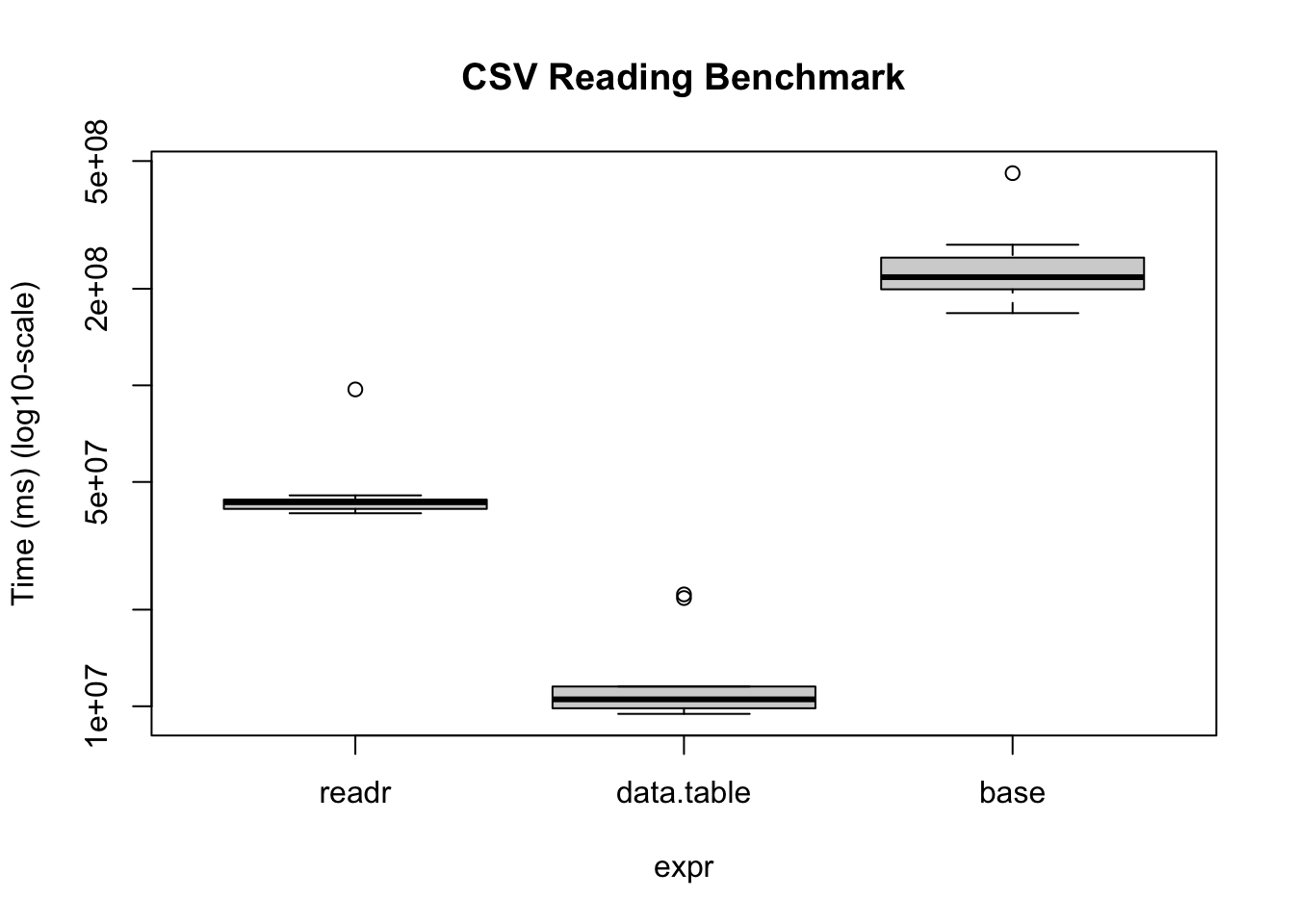
Under the hood, the readr package uses the vroom package. Nonetheless, there are some operations (dealing with character data mostly), where the vroom package shines. Regardless, data.table is a perfect alternative as it goes beyond just reading/writing data.

Example data manipulation

data.table is also the fastest for data manipulation. Here are a couple of examples aggregating data with data table vs dplyr

input <- if (file.exists("flights14.csv")) {
   "flights14.csv"
} else {
  "https://raw.githubusercontent.com/Rdatatable/data.table/master/vignettes/flights14.csv"
}

# Reading the data
flights_dt <- fread(input)
flights_tb <- read_csv(input, show_col_types = FALSE)

library(dplyr)

Attaching package: 'dplyr'

The following objects are masked from 'package:data.table':

    between, first, last

The following objects are masked from 'package:stats':

    filter, lag

The following objects are masked from 'package:base':

    intersect, setdiff, setequal, union

# To avoid some messaging from the function
options(dplyr.summarise.inform = FALSE)

microbenchmark(
  data.table = flights_dt[, .N, by = .(origin, dest)],
  dplyr = flights_tb |>
    group_by(origin, dest) |>
    summarise(n = n())
)

Unit: milliseconds
       expr      min       lq     mean   median       uq      max neval
 data.table 4.451124 4.743495 5.689651 4.931603 5.372681 34.82372   100
      dplyr 6.605305 7.039392 7.875169 7.405256 7.844940 22.65771   100

DELPHI